FLUIDS

Compositional PVT

A full equation-of-state workbench in the browser. Split the plus fraction, check the lab report, match the experiments by regression, then hand one tuned fluid to every other module and to your simulator.

Cubic equations of state, each with a Peneloux volume shift
3
Critical-property correlations for the pseudo-components
4
Lab experiments simulated, from CCE to swelling
5
Saturation pressures against an independent code
0.01%
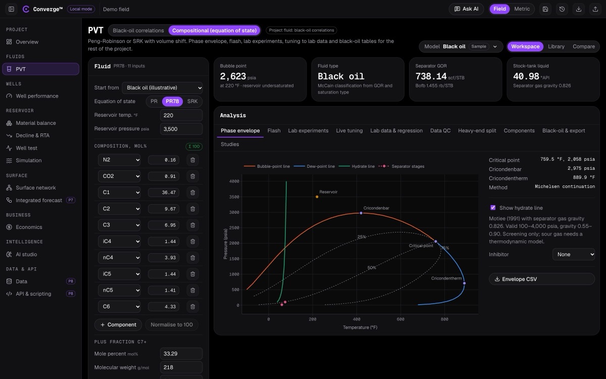
Converge compositional PVT screen: fluid composition table, saturation pressure and other readouts across the top, and a phase envelope with bubble-point, dew-point and quality lines.
Phase envelope for a sample fluid, with quality lines, the critical point and the cricondenbar and cricondentherm.
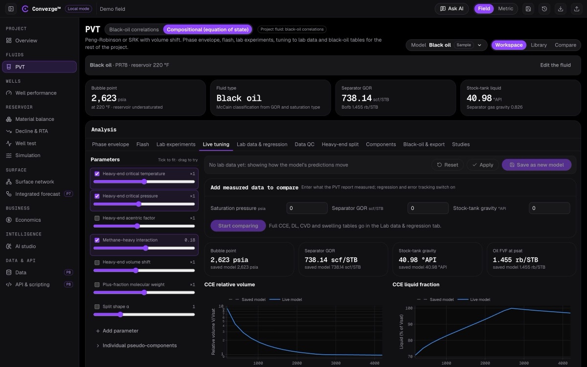
Converge live tuning screen: parameter sliders on the left, and saturation pressure, separator GOR and experiment plots that update as the sliders move.
Live tuning: move a parameter and the saturation pressure, separator GOR and experiment plots update.

WHAT IT DOES

From a lab composition to a tuned fluid model

Compositional PVT describes a reservoir fluid by its components and a cubic equation of state. You enter the composition from the lab report, with the plus fraction's molecular weight and specific gravity, and Converge splits the plus fraction into single carbon numbers, lumps them into pseudo-components and assigns critical properties and binary interaction parameters.

With the fluid described, Converge flashes it, traces the phase envelope and simulates the lab experiments: constant composition expansion, differential liberation, constant volume depletion, the multistage separator test and the swelling test. Each simulated table sits next to the measured one, so you can see where the model and the lab disagree.

Regression then adjusts the heavy-end, interaction and volume-shift parameters until the model reproduces the lab within the weights and bounds you set. The tuned model goes into the project's model library, and the one you pick becomes the project fluid that wells, reservoir, network and economics all read.
At a glance

  • Peng-Robinson 1976 and 1978, SRK, Peneloux volume shift
  • Whitson gamma split of the plus fraction, out to C200
  • Kesler-Lee, Riazi-Daubert, Twu and Pedersen critical properties
  • Michelsen stability test and Rachford-Rice flash
  • Phase envelope by Michelsen continuation
  • CCE, DL, CVD, multistage separator and swelling tests
  • Levenberg-Marquardt regression with bounds and weights
  • LBC and Pedersen corresponding-states viscosity
  • Minimum miscibility pressure by multiple mixing cell
  • Compositional grading with depth
  • Lab-data quality checks before tuning
  • Keyword-format compositional EOS deck export

KEY CAPABILITIES

The methods behind the workbench

Equations of state

Choose the cubic equation that suits the fluid and your company's practice. All three carry the Peneloux volume shift, which corrects liquid density without moving the phase equilibrium.

  • Peng-Robinson 1976
  • Peng-Robinson 1978, with the heavy-component correction for acentric factors above 0.49
  • Soave-Redlich-Kwong
  • Per-component Ωa and Ωb, available as regression parameters

Plus-fraction characterisation

The heavy end decides most of the fluid's behaviour, so every step of its description is visible and editable on the heavy-end split tab.

  • Whitson three-parameter gamma split, with mass conserved exactly
  • Lumping by equal mass, equal moles, custom carbon-number ranges or none
  • Critical properties by Kesler-Lee, Riazi-Daubert with Edmister acentric factor, Twu, or Pedersen et al.
  • Critical volume from Hall-Yarborough
  • Binary interaction parameters from typical values and Chueh-Prausnitz, with an interactive editor

Flash and phase behaviour

The flash is built to converge near the critical point, where gas condensates and volatile oils live.

  • Michelsen tangent-plane stability test
  • Rachford-Rice with a bounded Newton solve
  • Successive substitution with GDEM acceleration, switching to Newton near the critical point
  • Bubble and dew points bracketed by a stability scan, then refined by Newton
  • Phase envelope with quality lines and the critical point

Lab experiments and studies

Simulate the experiments in the lab report on the same basis the lab ran them, and run the studies a field development asks for.

  • Constant composition expansion and differential liberation
  • Constant volume depletion for gas condensates
  • Multistage separator test and separator optimisation
  • Swelling test for gas injection
  • Minimum miscibility pressure by multiple mixing cell, plus first-contact miscibility
  • Isothermal compositional grading with gas-oil contact detection
  • Cleaning of samples contaminated by oil-based mud

Regression and live tuning

Tune the model to the lab with control over what moves and by how much. Every run is kept, so you can compare runs and undo one.

  • Bounded Levenberg-Marquardt, with a Nelder-Mead fallback
  • Plus-fraction molecular weight, gamma shape, Tc, Pc and acentric-factor multipliers
  • Methane-heavy interaction, volume shift and single interaction pairs
  • Staged regression: saturation pressure first, then phase behaviour, then viscosity
  • Weights, bounds and per-point exclusion
  • Live tuning with sliders and a parameter advisor

Viscosity, hydrates and quality checks

Transport properties and screening checks come from the same fluid description, and the lab report is checked before any tuning starts.

  • Lohrenz-Bray-Clark viscosity with user coefficients, which can be regressed
  • Pedersen corresponding-states viscosity, with methane as the reference fluid
  • Hydrate screening by the Motiee correlation, with Hammerschmidt depression for methanol and MEG
  • About 40 lab-data checks, including the Hoffman plot, the Y-function, recombination and mass balance
  • Separate checks on the tuned model

WORKFLOW

How a fluid study runs in Converge

  1. Enter the composition

    Type or paste the mole fractions, the plus-fraction molecular weight and specific gravity, the reservoir temperature and the separator train.

  2. Describe the heavy end

    Pick the split, the lumping scheme and the critical-property correlation, and review the pseudo-components and interaction parameters.

  3. Check the lab report

    Run the data checks on the measured experiments, and exclude any point the checks or your judgement reject.

  4. Simulate and compare

    Trace the envelope and run the experiments. Each simulated table plots against the lab values.

  5. Tune to the lab

    Regress the parameters you choose, or move them by hand in live tuning, and compare runs side by side.

  6. Publish and export

    Save the model to the library, make it the project fluid, and export black-oil tables or a compositional deck.

VALIDATION

Checked against independent code and NIST data

The equation-of-state engine is compared with an independent open-source thermodynamics code on published fluids, and pure-component behaviour with NIST reference data. A dash means the benchmark reports the agreement rather than a pass threshold.

CheckReferenceConvergeTolerance
Bubble and dew points, SPE5 oil and a gas condensate, Peng-Robinson and SRKIndependent open-source codewithin 0.01%—
Two-phase flash compositionsIndependent open-source codewithin 10⁻⁵—
Pure-component vapour pressuresNIST reference datawithin 3%—
Plus-fraction split keeps the C7+ molecular weight (V8)218.0 g/mol218.0 g/mol10⁻⁶ g/mol

Not yet validated: a full phase envelope against a commercial package, and the minimum miscibility pressure calculation. The benchmarks page lists both.

INPUTS AND OUTPUTS

What goes in, what comes out

Inputs

  • Composition in mole percent, to C7+ or beyond
  • Plus-fraction molecular weight and specific gravity
  • Reservoir temperature and pressure
  • Separator train: stages, pressures and temperatures
  • Measured CCE, DL, CVD, separator and swelling data

Outputs

  • Saturation pressure and fluid type
  • Phase envelope with quality lines and the critical point
  • Simulated experiment tables beside the lab values
  • Match statistics for every regression target
  • Tuned models in the project's model library

Exports

  • Keyword-format compositional EOS deck (.inc)
  • EOS block in *-keyword format (.dat)
  • Separator-corrected black-oil tables: PVTO, PVDG, PVTW
  • PVTG and PVTO for wet gas and condensate
  • RSVD and RVVD initialisation tables
  • CSV of every table

FAQ

Compositional PVT: common questions

Which equations of state does Converge use?

Peng-Robinson 1976, Peng-Robinson 1978 and Soave-Redlich-Kwong. Each uses the Peneloux volume shift, which corrects liquid density without changing the phase equilibrium.

Can I tune the fluid model to my lab report?

Yes. Bounded Levenberg-Marquardt regression adjusts the plus-fraction, critical-property, interaction and volume-shift parameters you select, with weights, bounds and point exclusion. A staged mode fits saturation pressure first, then phase behaviour, then viscosity, and live tuning lets you move parameters by hand.

How is the plus fraction characterised?

By the Whitson three-parameter gamma distribution, out to C200 with mass conserved exactly. You then lump by equal mass, equal moles or custom ranges, and assign critical properties by Kesler-Lee, Riazi-Daubert, Twu or Pedersen.

What can I export to a reservoir simulator?

A keyword-format compositional EOS deck, an EOS block in *-keyword format, separator-corrected black-oil tables (PVTO, PVDG, PVTW, or PVTG and PVTO for condensates) and RSVD and RVVD initialisation tables, in field or metric units.

Does Converge model wax, asphaltene or hydrates rigorously?

Not yet. Hydrates are screened with the Motiee correlation and Hammerschmidt inhibitor depression, which is a screening check rather than a thermodynamic hydrate model. Wax and asphaltene models are not built.

Start with a fluid you know.