RESERVOIR

Reservoir simulation

A fully implicit, three-phase black-oil grid simulator that reads the project fluid directly. Build a grid or import a keyword-format deck, set wells and schedules, run it in the browser and read the maps, rates and convergence report.

Passes every published measure of the first SPE comparative project
SPE1
Material-balance closure on SPE1
9.3 × 10⁻⁸
SPE1 run time on one laptop core, 132 time steps
1.4 s
Cell limit for a model in this release
400,000
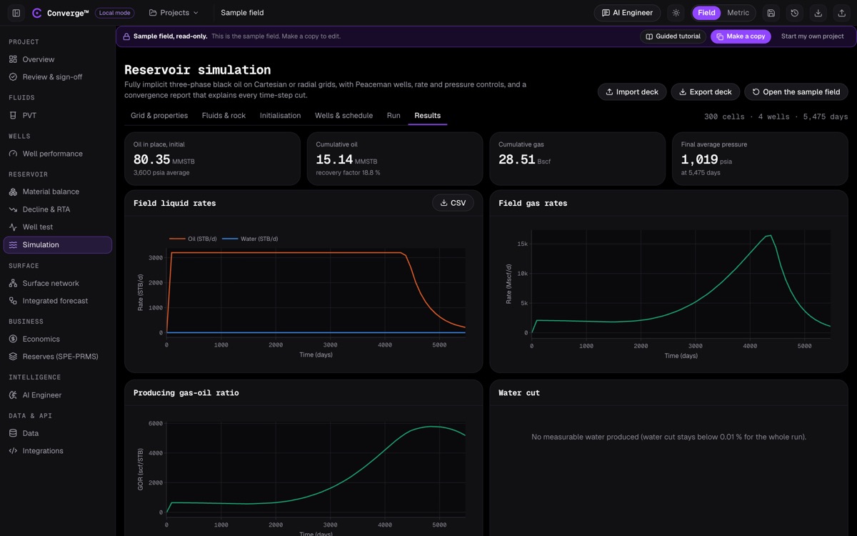
Converge reservoir simulation results: oil in place, cumulative oil and gas and final pressure across the top, with field liquid and gas rate and producing GOR plots against time.
Results for the sample field's coarse grid: field rates, cumulative production and producing GOR over 15 years.

WHAT IT DOES

A grid simulator on the same fluid as everything else

Reservoir simulation divides the reservoir into cells and solves mass conservation for oil, gas and water in each one through time. Converge's simulator is fully implicit: pressures and saturations are solved together at every time step, which keeps it stable at the large steps a field forecast needs.

Gas can be free, dissolved in the oil or carrying vaporised oil, and cells switch between those states as pressure crosses the saturation point (the Coats variable switching). The Jacobian comes from automatic differentiation, so it is exact, and each step reports its material-balance error.

The simulator reads the project fluid, tabulated at run time, or PVTO, PVDG and PVTW tables. It reads and writes a documented subset of a keyword-format simulator deck, lists any keyword it does not support rather than dropping it silently, and ships the SPE1 case built in.

At a glance

  • Fully implicit three-phase black oil
  • Two-point flux with upstream weighting
  • Coats variable switching, with vaporised oil (Rv)
  • Automatic-differentiation Jacobian
  • ILU(0)-preconditioned BiCGSTAB and GMRES
  • Appleyard chop and adaptive time steps
  • Cartesian and radial grids with active cells
  • Corey or tabulated relative permeability
  • Stone I, Stone II and Baker three-phase oil
  • Peaceman wells with rate and pressure controls
  • Equilibrium initialisation from contacts
  • Keyword-format deck import and export

KEY CAPABILITIES

Formulation, rock, wells and decks

Formulation and solver

A modern fully implicit formulation, with the convergence information an engineer needs to trust a run.

  • Fully implicit, finite volume, three-phase black oil
  • Two-point flux approximation with upstream weighting
  • Variable switching between free gas, dissolved gas and vaporised oil (Coats 1980)
  • Forward-mode automatic differentiation for the Jacobian
  • ILU(0) preconditioning with BiCGSTAB or restarted GMRES
  • Appleyard chop, adaptive time step and a convergence report that explains every cut

Grid and initialisation

Structured grids, initialised in equilibrium or uniformly.

  • Cartesian or radial grids
  • Active-cell flags
  • Equilibrium initialisation from contacts, with Rs and Rv against depth
  • Uniform initialisation for simple studies
  • Gaussian random permeability fields for demonstrations

Rock and fluid

Relative permeability, capillary pressure and PVT from your data or the project fluid.

  • Corey curves or tabulated relative permeability
  • Default saturation-weighted, Stone I (with Fayers-Matthews minimum oil saturation), Stone II or Baker three-phase oil
  • Oil-water and gas-oil capillary pressure
  • PVTO, PVDG and PVTW tables, or the project fluid tabulated at run time

Wells and schedules

The controls a field development plan uses, with economic limits.

  • Peaceman well index, including the anisotropic form
  • Producers on oil, gas, water, liquid or reservoir-volume rate with a minimum BHP, or on BHP
  • Water and gas injectors
  • Scheduled control changes and field oil-rate group control
  • Economic limits on oil rate, water cut and GOR

Decks and results

Bring a model in, take results and the deck out.

  • Reads and writes a documented keyword subset (.DATA)
  • Unsupported keywords listed back to you, never silently dropped
  • Pressure and saturation maps over time
  • Field and well rates, block pressures and the convergence report
  • Field results as CSV

Analytical checks

Quick physics checks beside the full simulation.

  • Buckley-Leverett frontal advance with the Welge tangent
  • SPE1 shipped built in, to compare against the published behaviour

WORKFLOW

Build, run and read a simulation

  1. Start a model

    Open SPE1, import a keyword-format deck, or build a grid with properties.

  2. Set rock and fluid

    Use the project fluid or PVT tables, and set relative permeability and capillary pressure.

  3. Initialise

    Set contacts and Rs or Rv against depth, or a uniform state.

  4. Add wells and a schedule

    Place producers and injectors, set controls, limits and schedule changes.

  5. Run

    Watch the time steps and the convergence report; the page stays usable while it runs.

  6. Read the results

    Step through pressure and saturation maps, field and well rates, and export the deck or CSV.

VALIDATION

SPE1 against the published behaviour

Odeh (1981), the first SPE comparative solution project: a 10 × 10 × 3 grid, one gas injector and one producer over ten years. Converge ships the case built in.

CheckReferenceConvergeTolerance
Oil-rate plateau20,000 STB/d20,000 STB/d1 STB/d
Producer switches from rate to pressure controlNear day 1,000Day 973Day 800 to 1,300
Peak average reservoir pressureNear 6,400 psia6,423 psia6,100 to 6,700 psia
Field oil rate, GOR, well BHP, block pressuresPublished reference run, 11 report times1% · 2.5% · 2% · 3%Worst difference shown
Material-balance closureMass conserved every step9.3 × 10⁻⁸Below 10⁻⁶ of pore volume
Buckley-Leverett water frontAnalytical Welge constructionWithin three cells—

Not built: compositional, thermal, polymer and CO₂ options; corner-point grids, faults and local refinement; deviated and multisegment wells; hysteresis; aquifer models in the simulator. The SPE9 match is partial and SPE3 has not been attempted. Performance above about 100,000 cells is not yet proven.

INPUTS AND OUTPUTS

What goes in, what comes out

Inputs

  • Grid dimensions and cell properties
  • Project fluid, or PVTO, PVDG and PVTW tables
  • Relative permeability and capillary pressure
  • Contacts and initial state
  • Wells, controls and schedule
  • Or a keyword-format deck

Outputs

  • Field and well rates and cumulatives
  • Pressure and saturation maps through time
  • Block pressures
  • Convergence report and material-balance error per step

Exports

  • Keyword-format simulator deck (.DATA)
  • sim-field.csv with field results
  • sim.run over the REST API and MCP

FAQ

Reservoir simulation: common questions

Is the simulator fully implicit?

Yes. Pressures and saturations are solved together each step, with Jacobians from automatic differentiation and a Newton loop with Appleyard chopping and adaptive time steps.

Can I import an existing simulation deck?

Yes, a documented subset of a keyword-format deck. Any keyword Converge does not support is listed back to you rather than ignored, and you can export the model as a deck.

Which three-phase relative permeability models are there?

The default saturation-weighted model, Stone I with the Fayers-Matthews minimum oil saturation, Stone II and Baker, on Corey curves or tables.

How big can a model be?

Up to 400,000 cells in this release. Performance above about 100,000 cells is not yet proven.

Is it compositional?

No. The simulator is three-phase black oil with dissolved gas and vaporised oil. Compositional fluids are tabulated into black-oil properties for it.

Run SPE1 in your browser.