RESERVOIR

Decline & RTA

Decline models fitted to production history, ranked by AIC, with P90/P50/P10 EUR from a bootstrap. Rate-transient analysis then reads permeability, fracture length and oil in place from the same rates and flowing pressures.

Decline models fitted and ranked on the same data
4
Agreement with an independent decline library
10⁻⁶
Bootstrap resamples by default
200
Flowing material balance against a known oil in place
1%
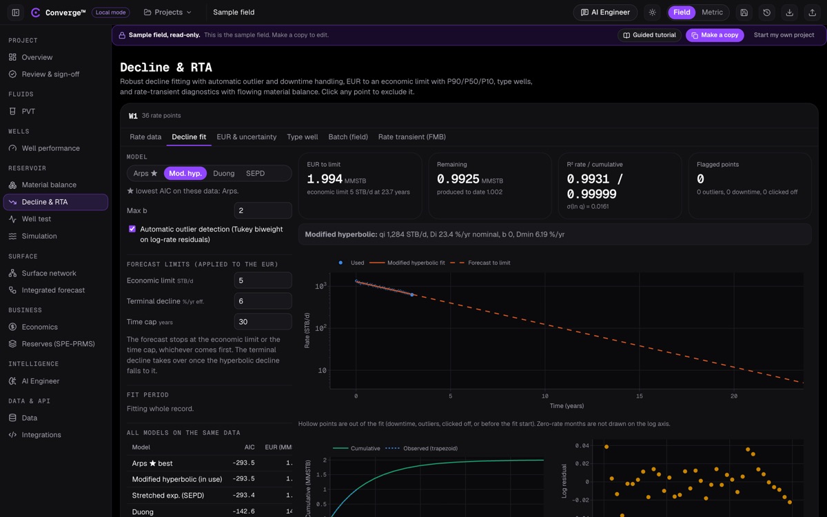
Converge decline fit screen: model choice and forecast limits on the left, EUR, remaining reserves and fit quality across the top, and the fitted decline and forecast on a log-rate plot.
A modified hyperbolic fit with its forecast to the economic limit, and all four models ranked by AIC.

WHAT IT DOES

Reserves from rates, without hiding the uncertainty

Decline curve analysis fits an empirical model to a well's rate history and extends it to an economic limit. Converge fits four models to the same data, by least squares on log rate, with outliers down-weighted and downtime excluded, and ranks them by the Akaike information criterion so a better score cannot come from extra parameters alone.

A single EUR hides the uncertainty, so Converge adds a block bootstrap: the residuals are resampled in blocks that keep month-to-month correlation, every resample is refitted, and the terminal decline is drawn around your input. The result is a P90, P50 and P10 EUR, and the spread between models is shown separately.

Rate-transient analysis goes further: with flowing pressures, rate-normalised pressure, Blasingame and Agarwal-Gardner plots, a type-curve match, linear-flow analysis and flowing material balance turn production data into reservoir properties.
At a glance

  • Arps exponential, hyperbolic and harmonic
  • Modified hyperbolic with a terminal decline
  • Duong for long linear flow
  • Stretched exponential (SEPD)
  • Tukey biweight outlier down-weighting
  • Ranking by AIC
  • Block-bootstrap P90/P50/P10 EUR
  • Change-point and level-shift detection
  • Type wells aligned at peak or first production
  • Batch decline across a field with a QC table
  • Blasingame and Agarwal-Gardner plots and type-curve match
  • Flowing material balance for oil and gas

KEY CAPABILITIES

Fitting, uncertainty and rate-transient analysis

Decline models

Four model families, all fitted to the same data so the comparison is fair.

  • Arps, with b from 0 (exponential) to above 1
  • Modified hyperbolic, switching to a terminal decline Dmin
  • Duong, for long transient linear flow
  • Stretched exponential production decline (SEPD)

Fitting

A fit that holds up on real, noisy production data.

  • Least squares on log rate
  • Tukey biweight down-weighting of outliers
  • Downtime detected and excluded
  • Differential evolution, then Nelder-Mead refinement
  • Click any point in or out of the fit
  • Fit from a chosen date, with a level-shift detector

EUR and uncertainty

EUR to the limits you set, with the uncertainty stated.

  • Economic limit, terminal decline and time cap
  • Models ranked by AIC; the best one is starred
  • Moving-block bootstrap of the residuals
  • Terminal decline drawn log-normally around your input
  • P90, P50 and P10 EUR, and the model-form spread shown apart

Type wells and batch decline

Work across a field, not one well at a time.

  • Type wells aligned at peak or first production
  • Outlier wells flagged, tails filled before averaging
  • Batch decline over many wells
  • A per-well QC table with flags
  • Batch results as CSV

Rate-transient analysis

Production data read as a long, variable-rate well test.

  • Rate-normalised pressure and its derivative
  • Blasingame plot with the harmonic stem
  • Agarwal-Gardner and normalised pressure integral plots
  • Type-curve match for an oil well in a closed circle, fitting permeability, area, skin and N
  • Square-root-of-time linear flow, giving xf√k

Flowing material balance

In-place volume from flowing data, without shutting the well in.

  • Oil flowing material balance (Agarwal-Gardner)
  • Gas flowing material balance (Mattar-McNeil)
  • Checks the volume from material balance

WORKFLOW

From a rate history to a reserves range

  1. Load the rates

    Paste rate history, or send it from the Data module with downtime already flagged.

  2. Fit the decline

    Fit all four models, review the AIC ranking and click out points that do not belong.

  3. Set the limits

    Enter the economic limit, terminal decline and time cap for the EUR.

  4. Run the bootstrap

    Get the P90, P50 and P10 EUR in the background while the page stays usable.

  5. Scale to the field

    Build type wells and run batch decline over every well, with QC flags.

  6. Read the reservoir

    Add flowing pressures for rate-transient analysis and flowing material balance.

VALIDATION

Synthetic wells with a known answer

The decline cases were generated from known parameters, so the truth is exact, and the rate and cumulative forms are checked against an independent open-source decline library. One coverage case is marginal, and the benchmarks page says so.

CheckReferenceConvergeTolerance
Arps fit to exact data, qi 3,500 STB/d, Di 60%/yr, b 0.70 (V15)The generating parametersRecovered exactly3 decimals
Arps fit with 3% noise (V15)The generating parametersRecovered5% on qi
Arps EUR to a 30-year cap (V16)4.78 MMSTB4.78 MMSTB0.005 MMSTB
Exponential and harmonic EUR (V17)1,980 and 9,210 STBClosed forms matched0.5 and 5 STB
Rate and cumulative, all four modelsIndependent decline libraryMatches10⁻⁶ relative
Oil flowing material balance (V14)Known synthetic truthWithin tolerance1%
Bootstrap P90–P10 contains the truth, 12 synthetic wells (V18)At least 80% coverage10 of 12, marginal80% coverage

Not built yet: type-curve matching for gas wells and Fetkovich type curves. Gas wells get diagnostics and flowing material balance.

INPUTS AND OUTPUTS

What goes in, what comes out

Inputs

  • Oil, gas or water rate history
  • Downtime or hours on
  • Flowing bottomhole pressure, for RTA
  • Project fluid properties
  • Economic limit, terminal decline and time cap

Outputs

  • Fitted parameters for each model and the AIC ranking
  • EUR and remaining reserves
  • P90, P50 and P10 EUR
  • Type-well profiles
  • Permeability, xf√k, skin and in-place volume from RTA

Exports

  • Batch decline CSV with the QC table
  • Decline forecast to Economics
  • Bootstrap P90/P50/P10 to Reserves

FAQ

Decline & RTA: common questions

Which decline model does Converge pick?

It fits Arps, modified hyperbolic, Duong and stretched exponential to the same data and stars the one with the lowest AIC. You can use any of them.

Do outliers and downtime spoil the fit?

No. Downtime is detected and excluded, outliers are down-weighted with a Tukey biweight, and you can click any point in or out.

How are P90, P50 and P10 EUR calculated?

By a moving-block bootstrap of the log-rate residuals, 200 resamples by default, each refitted with the same model, with the terminal decline drawn around your input. The spread between different models is reported separately.

Can I run decline on a whole field at once?

Yes. The batch tab fits every well, flags problems in a per-well QC table and exports the results as CSV. Type wells average aligned wells for new-well forecasts.

Does rate-transient analysis work for gas wells?

Diagnostics and gas flowing material balance (Mattar-McNeil), yes. The type-curve match is for oil wells in this release.

Put a range on every well's reserves.