RESERVOIR

Well test

Pressure-transient analysis from gauge data to a regressed analytical model. Read the Bourdet derivative, draw the straight lines, deconvolve the full rate history and fit a model with confidence intervals on every parameter.

Permeability recovered from a 180 md synthetic build-up
179.8 md
Confidence interval on every regressed parameter
95%
Boundary configurations, from a sealing fault to a closed rectangle
7
Deconvolution error on a multi-rate test
5%
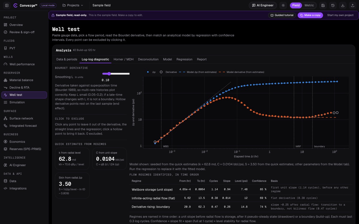
Converge well test log-log diagnostic: pressure change and Bourdet derivative on log axes, with wellbore storage, radial flow and boundary regimes marked, and quick estimates of permeability, storage and skin.
Log-log diagnostic on a build-up: storage, infinite-acting radial flow and a boundary, identified in time order.

WHAT IT DOES

Read the reservoir from a pressure record

A well test changes the rate and records how pressure responds. The shape of that response, read on a log-log plot of pressure change and its Bourdet derivative, tells you about wellbore storage, skin, permeability, boundaries, natural fractures and hydraulic fractures.

Converge takes the derivative against superposition time, so multi-rate histories plot correctly, flags end effects and names each flow regime in time order with a confidence. Quick estimates of permeability, storage and skin come straight from the regimes, and Horner and MDH straight lines confirm them.

You then build an analytical model from a well type, a reservoir type and a boundary, computed in Laplace space and inverted by Stehfest, and regress it to the data by Levenberg-Marquardt. Every fitted parameter comes with a 95% confidence interval, and deconvolution recovers the constant-rate response hidden in the whole rate history.
At a glance

  • Bourdet derivative on superposition time
  • Automatic flow-regime identification
  • Horner and MDH straight lines
  • Wellbore storage and skin, constant or changing (Fair)
  • Infinite-conductivity, finite-conductivity and uniform-flux fractures
  • Horizontal wells and partial penetration
  • Warren-Root and transient dual porosity
  • Two-zone radial composite
  • Faults, channels, closed rectangles and circles
  • Stehfest Laplace inversion
  • Levenberg-Marquardt regression with 95% intervals
  • Deconvolution of the full rate history

KEY CAPABILITIES

Diagnostics, models and regression

Diagnostics

The derivative and the regimes, before any model is chosen.

  • Bourdet derivative on superposition time, with a smoothing control
  • End-effect points shown hollow
  • Flow regimes named in time order, with slope, level and confidence
  • Quick permeability, storage and skin from the regimes
  • Shut-in periods detected from pressure alone

Straight-line analysis

The semilog methods engineers check by hand, done for you.

  • Horner plot, with the extrapolated pressure p*
  • MDH plot for drawdowns and early build-ups
  • Permeability and skin from the semilog slope

Well models

The near-well geometry, with constant or changing storage.

  • Vertical well with storage and skin
  • Infinite-conductivity, finite-conductivity and uniform-flux fractures
  • Horizontal well
  • Partial penetration
  • Changing wellbore storage (Fair)

Reservoir and boundary models

Heterogeneity and limits, combined freely with the well model.

  • Homogeneous
  • Warren-Root dual porosity, pseudo-steady state
  • Transient-slab dual porosity
  • Two-zone radial composite
  • Sealing fault, constant-pressure fault, channel
  • Closed rectangle, closed or constant-pressure circle

Regression and deconvolution

Fit the model to the data and say how sure the fit is.

  • Levenberg-Marquardt regression
  • Linearised 95% confidence interval on each parameter
  • Laplace-space solutions inverted by Stehfest
  • Deconvolution by von Schroeter, Hollaender and Gringarten, with Levitan's fitted initial pressure

Gas wells and reporting

Gas tests on the right basis, and a report that matches the screen.

  • Normalised pseudo-pressure for gas wells
  • Formation volume factor, viscosity and compressibility from the project fluid
  • A text report with the same numbers as the screen

WORKFLOW

From a gauge file to a fitted model

  1. Load the data and periods

    Paste the gauge record and rates. Shut-ins are found from the pressure, and you pick the period to analyse.

  2. Read the log-log plot

    Check the derivative, the regimes and the quick estimates of permeability, storage and skin.

  3. Draw the straight lines

    Confirm with Horner or MDH, and read p*.

  4. Deconvolve

    Recover the constant-rate response from the full rate history, to see further in radius.

  5. Build and regress the model

    Combine well, reservoir and boundary models, then regress them with confidence intervals.

  6. Report

    Write the report with the fitted values, intervals and plots.

VALIDATION

A synthetic build-up with a known answer

A 48-hour drawdown at 800 STB/d followed by 72 hours shut in, generated from the line-source solution with superposition. The known answer: k = 180 md, skin +4.5, initial pressure 3,650 psia.

CheckReferenceConvergeTolerance
Horner slope (V19)26.43 psi/cycle26.46 psi/cycle3%
Horner permeability (V19)180 md179.8 md3%
Extrapolated pressure p* (V20)3,650 psia3,650.0 psia2 psi
Skin, Horner (V21)+4.5+4.47±0.3
Permeability and skin, log-log derivative (V22)180 md, +4.5Within tolerance3%, ±0.3
Deconvolution of a multi-rate testKnown unit-rate responseRecovered5%, or 10% with 0.05 psi noise
Earlougher (1977) Example 5.1k = 12.8 md, skin 8.6Both matched5%

The model library is also checked against the published analytical limits of Theis, van Everdingen and Hurst, Gringarten, Ramey and Raghavan, Cinco-Ley and Samaniego, and Warren and Root.

INPUTS AND OUTPUTS

What goes in, what comes out

Inputs

  • Gauge pressure against time
  • Rate history
  • Net pay, porosity and wellbore radius
  • Formation volume factor, viscosity and total compressibility from the project fluid

Outputs

  • Permeability, skin and storage
  • Extrapolated and average pressure
  • Fracture, dual-porosity and boundary parameters
  • 95% confidence intervals
  • Deconvolved unit-rate response

Exports

  • Text report with every fitted value and interval
  • Horner analysis and derivative over the REST API and scripts

FAQ

Well test: common questions

Can Converge analyse multi-rate tests?

Yes. The derivative is taken against superposition time, so multi-rate histories plot correctly, and deconvolution recovers the constant-rate response from the whole history.

How reliable are the regressed values?

Each comes with a 95% confidence interval. The intervals are linearised, so they can understate the spread when parameters are strongly correlated, for example storage and skin.

Does it handle gas wells?

Yes, on normalised pseudo-pressure. Pseudo-time and rate-dependent skin are not built yet.

My gauge file has no rate column. Can I still use it?

Yes. Shut-in periods are detected from the pressure alone; you type the rates for each period.

Which reservoir models are available?

Homogeneous, Warren-Root and transient-slab dual porosity, and two-zone radial composite, with infinite, fault, channel, rectangle and circle boundaries. Multilayer models are not built yet.

Read your next build-up in Converge.