WELLS

Well performance

Inflow and outflow on the project fluid, with nodal analysis to find the operating point. Seven lift correlations are ranked against your well tests, and lift tables leave in the format your simulator reads.

Vertical-lift correlations, ranked against your well tests
7
Parameters for sensitivity runs
19
Beggs-Brill against two independent implementations
0.1%
Rate from a seeded Monte Carlo run
P90/P50/P10
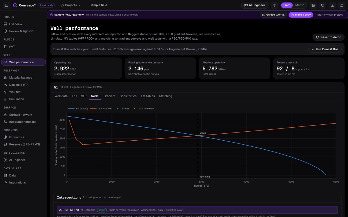
Converge well performance nodal screen: operating rate, flowing bottomhole pressure and absolute open flow across the top, and the inflow and outflow curves crossing at the operating point.
Nodal analysis on the sample well: the stable intersection of inflow and outflow, and the correlation that best matches the well tests.

WHAT IT DOES

Where the reservoir and the tubing agree

Well performance answers the question every production engineer starts with: how much will this well make, and what limits it? Converge builds the inflow performance relationship (IPR) from reservoir pressure and productivity, the vertical lift performance (VLP) from the tubing, deviation survey and temperature, and solves for the rate at which the two agree.

Every intersection is reported and flagged as stable or unstable, along with the minimum of the lift curve. A full pressure traverse shows where the losses are, split between gravity and friction. Sensitivities on up to 19 parameters show what moves the rate, and a seeded Monte Carlo run turns uncertain inputs into a P90, P50 and P10 rate with an influence ranking.

When you have well tests, Converge ranks all seven lift correlations against them, fits gravity and friction multipliers, checks against a gradient survey and fits the IPR, so the model you forecast with is the one that reproduces the field.
At a glance

  • PI, Vogel, composite, Fetkovich and Jones inflow
  • Darcy with skin, gas back-pressure and gas pseudo-pressure
  • Joshi horizontal-well inflow
  • Fracture and deviation equivalent skin
  • Beggs-Brill, Hagedorn-Brown, Gray, Duns-Ros, Orkiszewski and more
  • Linear or Ramey wellbore temperature
  • Nodal analysis with stability flags
  • Gas-lift performance curve and ESP stage curve
  • Gilbert, Ros, Baxendell and Achong chokes
  • Turner liquid-loading check
  • VFPPROD lift tables and CSV
  • Matching to well tests and gradient surveys

KEY CAPABILITIES

Inflow, lift and matching, method by method

Inflow performance

Pick the inflow model that suits the well and the data you have, from a single productivity index to back-pressure tests.

  • Productivity index, Vogel, and composite (Vogel below the bubble point)
  • Fetkovich and Jones (a, b) multi-rate models
  • Back-pressure C and n for gas wells
  • Darcy with skin, steady or pseudo-steady state
  • Gas pseudo-pressure (Al-Hussainy)
  • Joshi horizontal-well inflow

Skin

Total skin is built from its parts, so you can see what each contributes.

  • Hawkins damaged-zone skin
  • Cinco-Ley, Ramey and Miller deviation skin, with a warning above 75°
  • Cinco-Ley and Samaniego fracture equivalent skin, checked against the Prats limit
  • Non-Darcy skin, D times rate

Vertical lift

Seven multiphase correlations cover oil and gas wells, with the deviation survey and a temperature profile.

  • Beggs and Brill, with the Payne corrections
  • Hagedorn and Brown, with the Griffith bubble-flow correction
  • Gray, for gas and condensate wells
  • Duns and Ros, Orkiszewski, Aziz-Govier-Fogarasi and no-slip
  • Linear or Ramey (1962) wellbore temperature

Nodal analysis and sensitivities

The operating point, and what would move it.

  • Every IPR and VLP intersection, flagged stable or unstable
  • VLP minimum, the edge of stable flow
  • Gradient traverse with the gravity and friction split
  • Sensitivities on 19 parameters, from water cut to tubing size
  • Monte Carlo P90, P50 and P10 rate, with Spearman influence ranking

Artificial lift, chokes and loading

Screen lift options and surface limits on the same well model.

  • Gas lift: rate against injection, with the technical and economic optimum
  • ESP: your head-per-stage curve, scaled by the affinity laws and the stage count
  • Wellhead chokes by Gilbert, Ros, Baxendell and Achong, in critical flow
  • Turner et al. (1969) critical rate for liquid loading, shown on the VLP plot

Matching and lift tables

Calibrate the model to the field, then hand it to the simulator.

  • All seven correlations ranked against your well tests, the best one applied in a click
  • Gravity and friction multipliers fitted within 0.5 to 1.5
  • Check against a measured gradient survey
  • IPR fitted from well tests
  • VFPPROD lift tables over rate, THP, water fraction, gas fraction and lift gas

WORKFLOW

From well data to an operating point

  1. Describe the well

    Enter the deviation survey, tubing, temperature, wellhead conditions or choke, and any lift.

  2. Build the inflow

    Choose the IPR model, reservoir pressure, productivity and skin, or fit them from tests.

  3. Build the outflow

    Pick a lift correlation, or let the matching tab rank all seven against your tests.

  4. Solve the nodal point

    Read the operating rate, its stability and the VLP minimum, then the pressure traverse.

  5. Test what changes it

    Run sensitivities and the Monte Carlo rate, and screen gas lift or an ESP.

  6. Export lift tables

    Write VFPPROD and CSV lift tables for the simulator, and gradient CSV.

VALIDATION

Lift correlations checked against independent implementations

No textbook worked example with a stated answer exists for these correlations, so they are compared with independent open-source implementations, and the single-phase traverse with the exact answer. A dash means the benchmark reports the agreement rather than a pass threshold.

CheckReferenceConvergeTolerance
Beggs and Brill (1973)Two independent implementations, 14 flow stateswithin 0.1%—
Gray (1974)Two independent implementations, 14 flow stateswithin 0.2%—
Duns and Ros (1963)Independent implementation, bubble, slug and mist flowwithin 1%—
Whole gas-well traverse, 10,000 ft, dry and wetIndependent implementation0.02–0.18%—
Single-phase liquid traverse, deviated wellExact hydrostatic plus Colebrook frictionwithin 10⁻⁹—
Hydrostatic gradient in the well model (V23)18.06 lbm/ft³ gives 0.1254 psi/ft0.1254 psi/ft10⁻⁴ psi/ft

Hagedorn-Brown, Orkiszewski and Aziz-Govier-Fogarasi are implemented but not yet on the benchmarks page.

INPUTS AND OUTPUTS

What goes in, what comes out

Inputs

  • Project fluid, black-oil or compositional
  • Deviation survey and tubing description
  • Reservoir pressure, productivity and skin
  • Wellhead pressure or choke size
  • Well tests and gradient surveys
  • Gas-lift rate or ESP stage curve

Outputs

  • Operating rate and flowing bottomhole pressure
  • Absolute open flow
  • Stability flags and VLP minimum
  • Pressure and temperature traverse
  • Sensitivity plots and Monte Carlo P90, P50 and P10 rate
  • Correlation ranking against tests

Exports

  • VFPPROD lift-table keyword file (.inc), field units
  • Lift-table CSV
  • Gradient traverse CSV

FAQ

Well performance: common questions

Which lift correlation should I use?

Enter your well tests and Converge ranks all seven correlations by average error against them, then applies the best one in a click. You can fit gravity and friction multipliers on top.

Can I export lift curves for a reservoir simulator?

Yes. Converge writes VFPPROD lift tables over rate, tubing-head pressure, water fraction, gas fraction and lift-gas rate, in field units, plus the same tables as CSV.

Does it model horizontal and fractured wells?

Horizontal wells use the Joshi inflow model. Hydraulically fractured wells are modelled through the Cinco-Ley and Samaniego fracture equivalent skin, checked against the Prats limit. Transient and multi-fracture inflow models are not built yet.

How does Converge handle uncertainty in the well model?

A seeded Monte Carlo run samples the uncertain inputs and reports P90, P50 and P10 rate, with a Spearman ranking of which inputs matter most.

Can I design gas lift or an ESP?

You can screen both. Gas lift gives the rate against injection curve with its technical and economic optimum. The ESP uses your head-per-stage curve, scaled for frequency by the affinity laws. Valve spacing and pump catalogue sizing are not part of the module.

Find the operating point in minutes.