RESERVOIR

Material balance

Tank models on the project fluid, from diagnostic plots to an aquifer history match and a forecast. When the data cannot support an answer, Converge says so instead of printing a number.

Aquifer models, from pot to Carter-Tracy
5
Perturbed refits behind the P90/P50/P10 band
300
Oil in place against a known-answer tank
0.07%
Textbook examples reproduced, influx and withdrawal
2
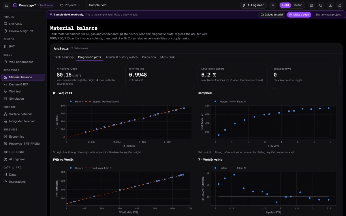
Converge material balance diagnostic screen: oil in place from the Havlena-Odeh line, R squared and drive-index closure across the top, and four diagnostic plots below.
Diagnostic plots on the sample tank: Havlena-Odeh, Campbell, F/Et against We/Et, and the drive-index closure.

WHAT IT DOES

Oil and gas in place from pressure and production

Material balance treats the reservoir as a tank: what came out, plus the expansion of what remains, must equal what was there to begin with, plus any water that flowed in. Paste the pressure and production history, and Converge computes the underground withdrawal F and the expansion terms from the project fluid, then plots them the ways that reveal the drive mechanism.

The Havlena-Odeh straight line gives the oil in place when the aquifer is right. Campbell and Cole plots show when it is not: a rising trend means influx not yet accounted for. You choose an aquifer model, and a global search fits its parameters while solving for N at every trial, so the match does not stall in a local minimum.

Every fit is checked for misfit, slope drift across the history and drive-index closure. A fit that fails is labelled not reliable, with the reasons, rather than shown as an answer. Randomised refits give a P90, P50 and P10 on the in-place volume, and the accepted tank predicts forward with relative permeability and a rate target.
At a glance

  • Oil tanks with gas cap, water and rock compressibility
  • Gas tanks, and condensate on a wet-gas basis
  • Havlena-Odeh, Campbell, Cole and p/Z plots
  • Drive indices with a closure check
  • Pot, Schilthuis, Fetkovich, van Everdingen-Hurst and Carter-Tracy aquifers
  • Radial and linear aquifer geometry
  • Differential-evolution history match
  • P90/P50/P10 from 300 randomised refits
  • Reliability check that blocks a bad fit
  • Tarner-Muskat prediction with Corey or tabulated relative permeability
  • Multi-tank with transmissibility links
  • Send to Economics

KEY CAPABILITIES

Tanks, plots, aquifers and prediction

Tank models

One tank formulation for each fluid type, all reading the project fluid.

  • Oil tank with initial gas cap ratio m
  • Water and rock compressibility terms
  • Gas tank
  • Condensate tank on a wet-gas equivalent basis
  • Drive indices for solution gas, gas cap, compaction and water drive

Diagnostic plots

The classic straight-line forms, each clickable to exclude a point.

  • F against Et, the Havlena-Odeh straight line through the origin
  • F/Eo against Eg/Eo for gas-cap size
  • F/Et against We/Et for the aquifer
  • Campbell plot and (F − We)/Et against Np
  • Cole plot and p/Z straight line for gas tanks

Aquifer models

Five influx models, from the simplest to the full unsteady-state solution.

  • Pot aquifer
  • Schilthuis steady state
  • Fetkovich pseudo-steady state, radial or linear
  • van Everdingen-Hurst unsteady state, radial or linear, by Stehfest inversion rather than tables
  • Carter-Tracy

History match and reliability

A global search finds the aquifer parameters; the in-place volume is solved exactly at every trial.

  • Differential-evolution search over the aquifer parameters
  • N solved linearly at each trial
  • Misfit, half-history slope drift and drive-index closure checks
  • A failing fit is shown as not reliable, with reasons
  • Randomised maximum likelihood: 300 refits perturbing pressures, initial pressure, PVT and rock compressibility

Prediction

The matched tank forecasts forward under a rate target and a pressure floor.

  • Tarner-Muskat style prediction
  • Rate target with a minimum pressure
  • Corey relative permeability
  • Imported SWOF and SGOF tables, with Baker three-phase oil
  • Forecast sent to Economics with one click

Multi-tank

Connect compartments that communicate through faults or a shared aquifer.

  • Implicit transmissibility links between tanks
  • Oil-oil and gas-gas connections
  • Each tank keeps its own aquifer and history

WORKFLOW

From history to a defensible in-place volume

  1. Load the tank and history

    Paste pressure and cumulative production, with unit-aware headers, or send it from the Data module.

  2. Read the diagnostic plots

    Check the Havlena-Odeh line and the Campbell and Cole trends, and click out any doubtful point.

  3. Match the aquifer

    Pick an aquifer model and run the history match. Review the reliability checks and the P90/P50/P10 band.

  4. Accept the match

    Accept a fit that passes; the in-place volume and aquifer go forward to prediction.

  5. Predict

    Set a rate target, pressure floor and relative permeability, and run the forecast.

  6. Share the forecast

    Send the profile to Economics, Reserves or the integrated forecast.

VALIDATION

Tested on tanks whose answer is known

The synthetic tanks were built from a known oil in place, so the truth is exact. Two textbook examples check the aquifer influx and the withdrawal arithmetic.

CheckReferenceConvergeTolerance
Volumetric tank built from N = 45 MMSTB, no aquifer (V10)45.00 MMSTB45.03 MMSTB1%
The same tank with an aquifer it does not have (V11)No wrong answer shownFit blocked as not reliable—
History match on the sample tank (V12)150 MMSTBWithin tolerance3%
P90–P10 band contains the truth (V13)150 MMSTB inside the bandBand contains the truthAt least 80% coverage over 10 histories
Infinite radial aquifer influx, Ahmed (2006) Example 10-4Constant and influx at 6 and 12 monthsReproduced0.5%
Underground withdrawal F, every row, Ahmed (2006) Example 11-1Published tableReproduced0.01 MMbbl

Multi-tank transmissibility links are entered in rb/d/psi in this release, and links carry no gravity or capillary terms.

INPUTS AND OUTPUTS

What goes in, what comes out

Inputs

  • Project fluid PVT
  • Pressure history
  • Cumulative oil, gas and water production
  • Water and gas injection
  • Rock and water compressibility
  • Aquifer geometry and properties

Outputs

  • Oil or gas in place, with P90, P50 and P10
  • Gas-cap ratio and aquifer parameters
  • Drive indices
  • Reliability verdict with reasons
  • Production and pressure forecast

Exports

  • Forecast sent to Economics
  • Tank available to Reserves and the integrated forecast

FAQ

Material balance: common questions

Will material balance give me a wrong oil in place without warning?

No. Every fit is checked for misfit, slope drift across the history and drive-index closure. A fit that fails is labelled not reliable and the reasons are shown, instead of an answer.

Which aquifer models are supported?

Pot, Schilthuis, Fetkovich, van Everdingen-Hurst and Carter-Tracy. Fetkovich and van Everdingen-Hurst can be radial or linear, and van Everdingen-Hurst is computed by Stehfest inversion rather than read from tables.

How is uncertainty in oil in place estimated?

By randomised maximum likelihood: 300 refits that perturb the pressures, initial pressure, PVT and rock compressibility. The spread gives the P90, P50 and P10.

Can I use my own relative permeability in the prediction?

Yes. Use Corey curves, or paste SWOF and SGOF tables; three-phase oil uses the Baker model.

Does it handle gas and condensate reservoirs?

Yes. Gas tanks have Cole and p/Z plots. Condensate tanks are handled on a wet-gas equivalent basis.

Find out what the tank is telling you.